Bradley-Terry Model

The Bradley-Terry Model is the standard approach for analyzing binary pairwise data. This applies to our problem because each data instance represents a binary outcome (whether team1 won the game) on a pair of teams. We use Bradley-Terry model to estimate the level of each team and to estimate the winning probabilities for the tournament games. Furthermore, we do this using Bayesian inference which helps capture the uncertainty in our predictions and provide useful insight.

TLDR:

• Estimated team levels and comparison with tournament seeds
• Predicted win probabilities for tournament games
• Predictive performance by log-loss curve

Table of Contents

• 1. Model
  • 1.1. Full Bayesian Model Statement
• 2. Implementation
  • 2.1. Setup
  • 2.2. Stan
• 3. Results
  • 3.1. Estimate of team levels
  • 3.2. Estimated Levels by Seed
  • 3.3. Winning Probabilities
  • 3.4. Log Loss Curve
• 4. Discussion
  • 4.1. So what have we gained from all this work?
  • 4.2. Next Steps

1 Model

Bradley-Terry Model assumes that the probability of winning, denoted \(\pi\), depends on the level of each team, denoted \(\alpha\). The goal is to estimate \(\alpha\) for every team using the outcome of the regular season games. Positive \(\alpha\) means that the team has a winning influence, negative means losing influence, and zero means that a team is neutral.

For (a potentially new) game \(i\) between team \(j[i]\) and team \(k[i]\), we'll estimate the winning probability for team \(j[i]\) as:

\[\pi_i = P(j[i] \text{ win}) = \frac{\exp(\alpha_{j[i]} - \alpha_{k[i]})}{\exp(\alpha_{j[i]} - \alpha_{k[i]}) + 1}\]

Here's a table to put things in perspective:

Difference in Levels (\(\alpha_{j} - \alpha_{k}\))	Probability of Winning (\(\pi_i\))	Odds of Winning (\(\frac{\pi_i}{1-\pi_i}\))
0	50%	1:1
0.7	67%	2:1
1.1	75%	3:1
1.6	83%	5:1
2.0	88%	7.5:1
3.0	95%	20:1
4.0	98%	55:1
5.0	99.3%	150:1

1.1 Full Bayesian Model Statement

Here we state the model in more detail for those interested. Bradley-Terry model can be seen as a logistic regression onto the level of each team.

1.1.1 Data Likelihood (Logistic Regression)

\[y_i \sim Bernoulli(\pi_i)\] \[\text{logit}(\pi_i) = \alpha_{j[i]} - \alpha_{k[i]}\]

1.1.2 Priors

For full Bayesian inference, we need to set a prior distribution for the unknown parameters. We'll start with a normal prior on the levels:

\[\alpha \sim N(0, \sigma^2)\]

According to this prior, an average team has a neutral effect on the outcome of the game. About 68% of teams have levels within 1 standard deviation away from being neutral, and about 95% of teams within 2 deviations.

We start with a noninformative uniform hyperprior on \(\sigma\).

1.1.3 Notation

• \(T\): total number of teams in the season
• \(j[i] \in \{1,...,T\}\): ID of team1 in game \(i\)
• \(k[i] \in \{1,...,T\}\): ID of team2 in game \(i\)
• \(y_i = \begin{cases} 1 & \text{ if team1 wins game } i\\ 0 & \text{ otherwise}\end{cases}\)
• \(\pi_i\): probability that team1 wins game \(i\)
• \(\alpha_{j[i]}, \alpha_{k[i]}\): level of team1 and team2 on winning the game

2 Implementation

We "fit" the model by sampling from the posterior distribution using MCMC in stan. In simple terms, we simulate thousands of scenarios of the world based on the observed data. We'll use the model parameters generated from each scenario to perform inference and prediction.

2.1 Setup

2.1.1 import

import pandas as pd
import numpy as np
from matplotlib import pyplot as plt
import matplotlib.patches as mpatches
import seaborn as sns
from src import utils  # see src/ folder in project repo
from src.data import make_dataset
import pystan
from sklearn.metrics import log_loss
import pickle

2.1.2 Helper Functions

print_df = utils.create_print_df_fcn(tablefmt='html');
show_fig = utils.create_show_fig_fcn(img_dir='models/bradley_terry/');

2.1.3 Load Data

data = make_dataset.get_train_data_v1(2015)
print_df(data.head())

	season	daynum	numot	tourney	team1	team2	score1	score2	loc	team1win	seed1	seednum1	seed2	seednum2	seeddiff	ID
0	2015	11	0	0	1103	1420	74	57	1103	1	nan	nan	nan	nan	nan	2015_1103_1420
1	2015	11	0	0	1104	1406	82	54	1104	1	nan	nan	nan	nan	nan	2015_1104_1406
2	2015	11	0	0	1112	1291	78	55	1112	1	Z02	2	nan	nan	nan	2015_1112_1291
3	2015	11	0	0	1113	1152	86	50	1113	1	nan	nan	nan	nan	nan	2015_1113_1152
4	2015	11	0	0	1102	1119	78	84	1119	0	nan	nan	nan	nan	nan	2015_1102_1119

2.1.4 Process Data

teams = set(data['team1'].unique()).union(data['team2'].unique())
team_f2id = dict(enumerate(teams, 1))  # start from 1 for stan's one-based indexing
team_id2f = {v:k for k, v in team_f2id.items()}

2.2 Stan

2.2.1 Model

model_code = '''
data {
  int<lower=0> T;
  int<lower=0> N;  // number of games in regular season
  int<lower=0> N_tourney;  // number of games in tournament
  int<lower=1, upper=T> j[N + N_tourney];  // index for team 1
  int<lower=1, upper=T> k[N + N_tourney];  // index for team 2
  int<lower=0, upper=1> team1win[N];
}

transformed data {

}

parameters {
  real alpha[T];
  real<lower=0> sigma;  // variance for team levels
}

transformed parameters {
  real<lower=0, upper=1> pi[N_tourney];  // probability that team1 wins
  for(n in 1:N_tourney) {
    pi[n] = inv_logit(alpha[j[N+n]] - alpha[k[N+n]]);
  }
}

model {
  vector[N] theta;  // logits
  alpha ~ normal(0, sigma);
  for(n in 1:N)
    theta[n] = alpha[j[n]] - alpha[k[n]];
  team1win ~ bernoulli_logit(theta);
}

generated quantities {

}
'''
sm = pystan.StanModel(model_code=model_code)

2.2.2 Data

stan_data = {
    'T': len(teams),
    'N': (data.tourney == 0).sum(),
    'N_tourney': (data.tourney == 1).sum(),
    'j': data['team1'].map(team_id2f).values,
    'k': data['team2'].map(team_id2f).values,
    'team1win': data.loc[data.tourney == 0, 'team1win'].values
}

2.2.3 Sample from the Posterior

fit = sm.sampling(data=stan_data, iter=1000, chains=4)
with open("bradley-terry.pkl", "wb") as f:
    pickle.dump({'model_code': model_code, 'sm': sm, 'fit': fit}, f, protocol=-1)

2.2.4 Model Diagnostics

It's important to check that MCMC algorithm converged. This is done offline to avoid clutter.

3 Results

3.1 Estimate of team levels

la = fit.extract(permuted=True)  # extract MCMC samples
alpha = la['alpha']  # estimated team levels
tourney_teams = list(set(data.loc[data['tourney'] == 1, ['team1', 'team2']].values.flatten()))
tourney_teamsf = [team_id2f[t]-1 for t in tourney_teams]  # subtract 1 for zero-based indexing
team_seeds = pd.DataFrame(np.vstack([data[['team1', 'seednum1']].dropna().values,
                                     data[['team2', 'seednum2']].dropna().values])
                          .astype(int), columns=['team', 'seed']).drop_duplicates()
fig, axes = plt.subplots(2, 1, sharex=True)
bins = np.arange(-4, 5, 0.5)
axes[0].hist(np.mean(alpha, axis=0), edgecolor='black', bins=bins);
axes[1].hist(np.mean(alpha[:, tourney_teamsf], axis=0), edgecolor='black', bins=bins);
axes[0].set_title('All Teams', loc='left')
axes[1].set_title('Tournament Teams', loc='left')
axes[1].set_xlabel('Estimated Level')
for i in range(2):
    # axes[i].grid(axis='x')
    axes[i].axvline(0, c='r')
plt.suptitle('Estimated Level of Teams')
show_fig('average_team_levels.png')

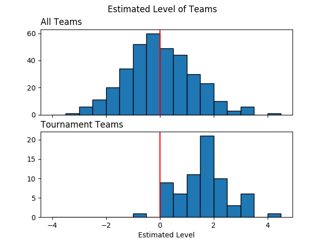
This figure gives us a few insights about our model. Point 1 below suggests that the model is generally learning the right pattern. Points 2 and 3 might indicate lack of fit and a potential direction for model expansion.

1. Most of the tournament teams have high estimated levels. It looks like all teams with estimated level beyond 2.5 have made it to the tournament.
2. One of the tournament teams has a negative estimated level. What is this team and how did they make it to the tournament? Before we do a deep dive, there's a few possibilities:
   • the team had an extremely competitive conference and lost many games.
   • the team qualified in a non-traditional way (maybe by winning a qualifying tournament through a series of upsets?). I have no idea how this process works.
3. According to the model, there are several teams that didn't make the tournament even though they are better than some of the qualifying teams. For instance, over 30 teams had an estimated level between 1 and 1.5. However, among qualifying teams, there's only about 10 teams in that range while about 15 teams have levels less than 1.0.

3.2 Estimated Levels by Seed

team_levels = (pd.DataFrame({
    'alpha_mean':np.mean(alpha[:, tourney_teamsf], axis=0),
    'alpha_l05':np.quantile(alpha[:, tourney_teamsf], 0.05, axis=0),
    'alpha_l25':np.quantile(alpha[:, tourney_teamsf], 0.25, axis=0),
    'alpha_median':np.quantile(alpha[:, tourney_teamsf], 0.50, axis=0),
    'alpha_u75':np.quantile(alpha[:, tourney_teamsf], 0.75, axis=0),
    'alpha_u95':np.quantile(alpha[:, tourney_teamsf], 0.95, axis=0),
    }, index=tourney_teams)
                .pipe(pd.merge, team_seeds, left_index=True, right_on='team')
                .pipe(lambda x: x.sort_values(['seed', 'alpha_mean'], ascending=[True, False]))
)


error_bars_50 = [team_levels['alpha_mean'] - team_levels['alpha_l25'],
                 team_levels['alpha_u75'] - team_levels['alpha_mean']]
error_bars_95 = [team_levels['alpha_mean'] - team_levels['alpha_l05'],
                 team_levels['alpha_u95'] - team_levels['alpha_mean']]
fig, ax = plt.subplots(figsize=(10, 5))
x = team_levels['seed'].values + np.tile([-0.33, -0.17, 0.17, 0.33], 17)
ax.errorbar(x, team_levels['alpha_mean'], yerr=error_bars_95, fmt='none', c='r', label='90% interval', lw=0.5)
ax.errorbar(x, team_levels['alpha_mean'], yerr=error_bars_50, fmt='none', c='k', label='50% interval', lw=2.5)
ax.scatter(x, team_levels['alpha_mean'], c='k', label='mean level')
ax.set_xlabel('Seed')
ax.set_ylabel('Estimated Level')
ax.axhline(0, color='k', linestyle='--', lw=0.5)
ax.set_title('Estimated Levels by Seed')
ax.legend()
show_fig('estimated_levels_by_seed.png')

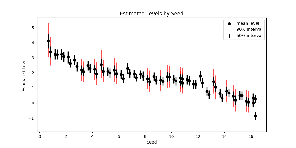
How can we check that our estimates are good? One way is to compare our estimates against the tournament seeds. The figure above confirms that the two are in agreement. Note that seeds are assigned within conference (or region?) so four teams share the same seed.

There's some separation in estimated levels among the top two seeds from every conference, bottom (below 12) seeds, and the rest of the pack.

3.3 Winning Probabilities

pi = la['pi']
idx_sorted = np.argsort(np.median(pi, axis=0))
pi_sorted = pi[:,idx_sorted]
y_true = data.loc[data.tourney == 1, 'team1win'].values
y_pred = np.median(pi, axis=0) > 0.5
color_sorted = np.where(y_true == y_pred, 'b', 'r')[idx_sorted]
nrow = 9
ncol = 8
fig, axes = plt.subplots(nrow, ncol, figsize = (10, 10), sharex=True)
for row in range(nrow):
  for col in range(ncol):
    idx = row * ncol + col
    axes[row, col].set_yticklabels([])
    if idx < (y_true.shape[0]):
      axes[row, col].hist(pi_sorted[:,idx], bins=30, color=color_sorted[idx]);
blue_patch = mpatches.Patch(color='blue', label='Correct')
red_patch = mpatches.Patch(color='red', label='Error')
fig.legend(handles=[blue_patch, red_patch], loc='lower center')
plt.subplots_adjust(left=None, bottom=None, right=None, top=None, wspace=0.05, hspace=0.05)
plt.suptitle('Posterior Distribution of Winning Probabilities (2015 Tournament)')
show_fig('win_probabilities.png')

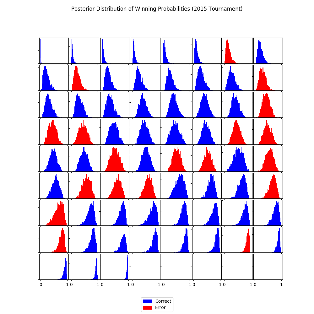
Here, we use our simulations to predict the winning probabilities. This is where we can leverage the power of Bayesian inference.

Each subplot above represents a tournament game and the histogram contains the predicted win probabilities (that team1 will win) over many simulated scenarios. For convenience, histograms are ordered by the median predicted win probability.

• symmetric and wide histogram means that the two teams are closely matched and it's difficult to predict who will win
• A skewed histogram means that one team is more likely to win than the other
• A narrow histogram means that the model is quite certain about the probability of winning

In order to check if the model is consistent with observed outcomes, I used the median predicted probability to decide whether or not team1 is predicted to win. Blue and red histograms indicate whether the model was correct or not, respectively. Few things to note here:

• When the model thinks the teams are closely matched (wide and centered histograms), the predictions go either way.
• When the model thinks there's a mismatch, it is correct more often than not.
• There's a small number of "upsets" when the model is very certain but wrong. We can deep dive into these games. Upsets can always happen, but we could gain new insights on how to expand the model.

3.4 Log Loss Curve

Let's evaluate the predictions over all seasons using the log-loss curve as we did for benchmark models. We can do this by creating a function that wraps around the essential part of the code for making the prediction. The code below takes a while and should ideally be run in parallel.

def evaluate(sm, season):
    data = make_dataset.get_train_data_v1(season=season)
    teams = set(data['team1'].unique()).union(data['team2'].unique())
    team_f2id = dict(enumerate(teams, 1))  # start from 1 for stan's one-based indexing
    team_id2f = {v:k for k, v in team_f2id.items()}
    stan_data = {
        'T': len(teams),
        'N': (data.tourney == 0).sum(),
        'N_tourney': (data.tourney == 1).sum(),
        'j': data['team1'].map(team_id2f).values,
        'k': data['team2'].map(team_id2f).values,
        'team1win': data.loc[data.tourney == 0, 'team1win'].values
    }
    fit = sm.sampling(data=stan_data, iter=1000, chains=4)
    la = fit.extract(permuted=True)  # extract MCMC samples
    pi = la['pi']
    y_true = data.loc[data.tourney == 1, 'team1win'].values
    return log_loss(y_true, np.median(pi, axis=0))

log_losses = []
seasons = range(1985, 2019)
for season in seasons:
    print('season = '.format(season))
    log_losses.append(evaluate(sm=sm, season=season))
with open("bradley-terry-logloss.pkl", "wb") as f:
    pickle.dump({'log_losses': log_losses, 'seasons':seasons}, f, protocol=-1)

Here is the resulting log-loss curve over all seasons.

fig, ax = plt.subplots()
log_loss_df = pd.read_csv('./log_loss_benchmark.csv').set_index('season')
log_loss_df['bradley-terry'] = log_losses
log_loss_df.plot(ax=ax)
ax.set_title('Comparison of Models by Log Loss')
ax.set_ylabel('Log Loss')
show_fig('log_loss.png')

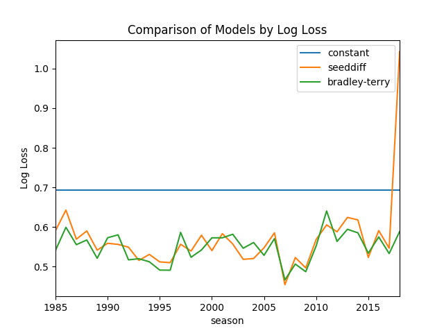
The predictive performance of Bradley-Terry model is comparable to the SeedDiff benchmark model. This is not surprising because they're using almost the same information.

4 Discussion

4.1 So what have we gained from all this work?

• A modeling framework

  As mentioned above, Bradley-Terry model is a special case of logistic regression. This is a model we can build on by adding additional features. We'll also be able to expand on the model by using hierarchical Bayesian models.

• Estimated levels of all teams

  While only the top 68 teams are seeded, we now have an estimate of the levels of every team in NCAA. We might be able to leverage this for future models.

• Insight about competitiveness

  The estimated levels of the teams gives us our first look at defining and quantifying competitiveness. The posterior histograms can also help visualize the competitiveness of the games.

4.2 Next Steps

4.2.1 Include additional features

Is there an effect of having won in a previous meeting during the season

• Does a pair of teams play each other more than once in a season?

4.2.2 Use score difference information

The current model estimates the team levels only based on whether a team won the game or not. For example, whether a team won by 20 points or 2 points is irrelevant for this model. We'll try to expand the model to account for this.

4.2.3 Allow parameters to vary by conference

We might expand the variance component to \(\sigma_{k[i]}^2\) where \(k\) indexes over conferences. This might help us compare the competitiveness of the conferences.

4.2.4 Use T-distribution as prior for team levels

Normal distribution can be restrictive. For example, it implicitly constrains the estimates so that 68% of the team levels are within one standard deviation, 95% within two, and so on. We might use a T-distribution (infinite mixture of normals) to build a more robust model.

4.2.5 Model the data-shift

An important question is whether there's any systematic difference between regular season games and tournament games. For example,

• does a team get better or more competitive during the tournament?
• does a team get less competitive at the end of regular season when they've secured a tournament seed?
• what happens to a team if a key player is injured at the end of the season and will miss the tournament?