Benchmark Models

No fancy machine learning models, here. Just a collection of simple and intuitive hacks. Later we'll need these benchmarks to understand if our fancy models are actually any good.

Quick Summary:

tournament seed seem like a decent predictor of who will win (LogLoss)
probabilities of 0 or 1 can ruin you

1. Setup
2. Models
- 2.1. Constant Model
- 2.2. SeedDiff Model
3. Evaluation
- 3.1. LogLoss

1 Setup

1.1 Load Packages

import pandas as pd
import numpy as np
from matplotlib import pyplot as plt
import seaborn as sns
from tabulate import tabulate
from sklearn.metrics import log_loss
from sklearn.metrics import roc_curve, auc
from src import utils  # see src/ folder in project repo
from src.data import make_dataset

1.2 Helper Functions

print_df = utils.create_print_df_fcn(tablefmt='html');
show_fig = utils.create_show_fig_fcn(img_dir='models/benchmark/');

1.3 Load Data

data = make_dataset.get_train_data_v1()
print_df(data.head())

	season	daynum	team1	team2	score1	score2	loc	team1win	seed1	seednum1	seed2	seednum2	seeddiff	ID
0	1985	20	1228	1328	81	64	0	1	W03	3	Y01	1	-2	1985_1228_1328
1	1985	25	1106	1354	77	70	1106	1	nan	nan	nan	nan	nan	1985_1106_1354
2	1985	25	1112	1223	63	56	1112	1	X10	10	nan	nan	nan	1985_1112_1223
3	1985	25	1165	1432	70	54	1165	1	nan	nan	nan	nan	nan	1985_1165_1432
4	1985	25	1192	1447	86	74	1192	1	Z16	16	nan	nan	nan	1985_1192_1447

2 Models

2.1 Constant Model

\[\text{All teams are created equal}\]

models = {}
models['constant'] = pd.DataFrame({'ID':data['ID'], 'Pred':0.5})

2.2 SeedDiff Model

\[\text{Higher seeded team is more likely to win}\]

In this model, we use the relative difference in seed to predict the winning team. For example,

If two teams have equal seeds, they have equal probabilities of winning.
If two teams have maximum difference in seeds (i.e. top seed vs bottom seed), then the team with higher (lower value) seed has winning probability of 1.

In math, this is \[d_i = \text{difference in seeds for game } i\] \[p(win_i) = \frac{d_i - d_{min}}{d_{max} - d_{min}}\]

models['seeddiff'] = (data.set_index('ID')
                      .pipe(lambda x:
                            ((x['seeddiff'] - x['seeddiff'].min()) /
                             (x['seeddiff'].max() - x['seeddiff'].min())))
                      .reset_index()
                      .rename({'seeddiff':'Pred'}, axis=1)
                      .dropna()
)

3 Evaluation

3.1 LogLoss

models_loss = {}
for m_name, m in models.items():
    m_loss = (m.pipe(pd.merge,
                     data.loc[data.tourney == 1, ['ID', 'team1win', 'season']],
                     on='ID', how='inner')
              .groupby('season')
              .apply(lambda x: log_loss(x['team1win'], x['Pred'])))
    models_loss[m_name] = m_loss
log_loss_df = pd.DataFrame(models_loss)
log_loss_df.to_csv('./log_loss_benchmark.csv')
fig, ax = plt.subplots()
log_loss_df.plot(ax=ax)
ax.set_title('Log Loss - Benchmark Models')
ax.set_ylabel('Log Loss')
show_fig('log_loss.png')
show_fig

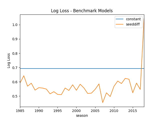
3.1.1 When a model is full of itself

There is a huge spike in 2018 season because a 16th seeded team beat the top seeded team. In this case, the SeedDiff Model predicts a winning probability of exactly 0, which would result in an infinite log-loss. Fortunately, sklearn.metrics.log_loss clips the predicted probabilities away from 0 and 1 by a small amount to prevent infinite loss. It'd be a good idea to prevent our models from predicting 0 or 1 probabilities (i.e. pretending to know the outcome with certainty).

Here is a query for the game that caused an infinite loss in SeedDiff Model.

tmp = data[(data.season == 2018) & (data.tourney == 1)]
print_df(tmp.loc[tmp.seeddiff.abs().sort_values(ascending=False).index].head())

	season	daynum	tourney	team1	team2	score1	score2	team1win	seed1	seednum1	seed2	seednum2	seeddiff	ID
158239	2018	137	1	1420	1438	74	54	1	Y16	16	Y01	1	-15	2018_1420_1438
158241	2018	137	1	1411	1462	83	102	0	Z16b	16	Z01	1	-15	2018_1411_1462
158225	2018	136	1	1347	1437	61	87	0	W16b	16	W01	1	-15	2018_1347_1437
158216	2018	136	1	1242	1335	76	60	1	X01	1	X16	16	15	2018_1242_1335
158236	2018	137	1	1168	1345	48	74	0	W15	15	W02	2	-13	2018_1168_1345

Table of Contents